An autonomous vehicle barrels down a rainy street, its neural net confidently forecasting the pedestrian’s path as a neat Gaussian blob—right up until the human slips sideways into traffic.
That’s the nightmare measuring divergence between actual and predicted distributions exposes, a shift ripping through machine learning like a fault line. We’ve outgrown the cozy era of point predictions, where accuracy or MSE sufficed for slapping labels on cats or guessing house prices. Now? Generative models, diffusion pipelines, trajectory forecasts—they spit out entire probability clouds. And if those clouds don’t hug reality’s shape, disaster lurks.
Why Accuracy Crumbles Under Modern Loads
Accuracy shines in simple classification—tick, image labeled, done. But toss in uncertainty, multimodality, the wild tails where black swans nest? It blindsides you.
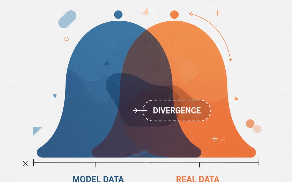
Two distributions may have the same mean yet have very different spreads, peaks, or modes. Ignoring this difference can lead to decisions that appear accurate but fail in practice.
Spot on. Imagine financial risk models: your algo nails the expected return but slims the loss tails to nothing. Boom—market crash, and you’re caught flat-footed. Or diffusion models churning pixels; mean color right, but the variance? Blurry mush instead of crisp edges. Here’s the thing—divergences don’t care about averages. They probe the full probabilistic guts.
Old-school ML was Newtonian: predict the position, fire. Today’s probabilistic physics demands the wave function. My take? This mirrors the 1930s quantum leap—point particles yielded to smeared clouds, birthing technologies we can’t unsee. Divergences force that maturity on AI, or we stay stuck in toy problems.
A three-word truth: Shape matters.
What Makes a Divergence Tick?
Divergences aren’t your grandma’s Euclidean distances. No symmetry, no tidy triangle inequality—just raw informational mismatch between true P(x) and model’s Q(x).
Take Kullback-Leibler, the granddaddy:
D_KL(P || Q) = ∫ p(x) log(p(x)/q(x)) dx
Asymmetric beast. It screams when Q ignores P’s mass, perfect for ensuring coverage—like in autonomous driving, where missing a rare swerve kills. Flip it to D_KL(Q || P), and it hugs P’s peaks, blind to tails. Subtle choice, massive stakes.
But KL hates zeros—q(x)=0 where p(x)>0? Infinity. Enter Jensen-Shannon, the polite cousin:
M = 0.5(P + Q) JSD(P, Q) = 0.5D_KL(P || M) + 0.5*D_KL(Q || M)
Symmetric, bounded (0 to 1 in bits), GANs’ secret sauce. It flags poor overlap without exploding, dodging mode collapse where generators pump identical fakes.
And Wasserstein? Earth Mover’s Distance. Piles of sand—how much dirt to shift? Symmetric metric, handles disjoint supports. In trajectories, it gauges path deviations geometrically, not just info-loss.
Choice boils down to worldview: info theorists grab KL/JS; geometers, Wasserstein.
Is KL Divergence Overhyped—or Underrated?
KL rules variational autoencoders, language models, Bayesian nets. Why? It quantifies “extra bits needed if Q fakes P.” Minimize it, and your approx stays faithful.
Yet asymmetry bites. In trajectory forecasting, KL(P||Q) blankets all plausible paths (safety win); KL(Q||P) trims to likely ones (efficiency). Pick wrong, and your self-driving rig either lags or blindsides.
Critique time: Companies hype KL-trained models as “uncertainty-aware,” but gloss over direction. It’s PR spin—train both ways, report the flattering one. Real fix? Hybrid losses, or we’re chasing ghosts.
Short para. KL endures.
Why Does Wasserstein Distance Feel Like the Future?
Optimal transport roots give it geometric intuition—move mass minimally. 1D: integral of CDF diffs. Higher-D: inf over couplings of p-norms.
Shines where supports mismatch: diffusion models morphing noise to images, pedestrian predictions leaping sidewalks. GANs love it too—Wasserstein GANs stabilized training, birthing sharper fakes.
Prediction: As multimodal gen-AI explodes (think video trajectories), Wasserstein surges. It’ll retrofit eval suites, much like cross-entropy dethroned MSE in classification. Architecturally? Forces pipelines to optimize transport plans, not just samplers—deeper shift than meets the eye.
How Do You Pick Your Divergence Weapon?
KL for info fidelity, JS for symmetry/stability, Wasserstein for shape. Test ‘em—compute on held-out data.
In practice? Libraries like SciPy, POT swallow the math. But interpret: low divergence ≠ deploy-ready. Pair with calibrated probs, domain sims.
Wander a bit: Remember early diffusion papers? They leaned Wasserstein to tame gradients. Now, hybrids blend all three. The why? No silver bullet—reality’s distributions defy purity.
One sentence. Experiment wildly.
The Hidden Architectural Overhaul
Divergences aren’t bolt-ons; they rewrite training. Point-pred models minimized deltas; now, full-dist evals demand richer architectures—flows, diffusers, ensembles.
Robustness jumps: rare events surface, trust metrics bloom. But compute? Oof—sampling-heavy. GPU farms groan.
Unique angle: This echoes econometrics’ 80s pivot from means to quantiles, averting ‘87 crash blindspots. ML follows suit, or faces its own reckoning.
🧬 Related Insights
- Read more: Medusa Ransomware: Zero-Days to Encryption in Under 24 Hours
- Read more: How Kubernetes Operators Are Cracking Open True Database Sovereignty with Portable Postgres
Frequently Asked Questions
What is Kullback-Leibler divergence used for?
KL measures info loss approximating one distribution with another—core in VAEs, policy gradients, ensuring models don’t miss probability mass.
How does Wasserstein distance differ from KL?
Wasserstein’s a true metric stressing geometry (mass movement cost), handles disjoint supports; KL’s asymmetric info-gap, blows up on zeros.
Why use divergence metrics over accuracy in ML?
Accuracy ignores distribution shape—vital for gen models, uncertainty; divergences catch tails, multimodality accuracy misses.